富士山をプロットする関数をみかけたので、Rで描いてみた。

fx <- function(x){x^4-x^2+6}
sfx <- function(x){12/(abs(x)+1)}
gx <- function(x){1/2*cos(6*x)+7/2}

plot(gx,-2,2,xlim=c(-7,7),ylim=c(0,7),xlab="",ylab="")
par(new=T)
plot(sfx,-7,-1,xlim=c(-7,7),ylim=c(0,7),axes=F,xlab="",ylab="")
par(new=T)
plot(sfx,1,7,xlim=c(-7,7),ylim=c(0,7),axes=F,xlab="",ylab="")
par(new=T)
plot(fx,-1,1,xlim=c(-7,7),ylim=c(0,7),axes=F,xlab="",ylab="")

ggplotで関数だけ描く方法わからんなぁとつぶやいたら、教えてもらったのでggplot2でも描いた。

gx <- function(x){
x[-2>x | x>2] <-NA
1/2*cos(6*x)+7/2
}

fx <- function(x){
x[x<(-1)] <- NA
x[x>1] <- NA
x^4-x^2+6
}

fx <- function(x){
x[-1<x & x<1] <-NA
12/(abs(x)+1)
}

ggplot(data.frame(x=c(-7,7),y=0), aes(x,y))+stat_function(fun=gx) \
+stat_function(fun=fx)+stat_function(fun=sx)

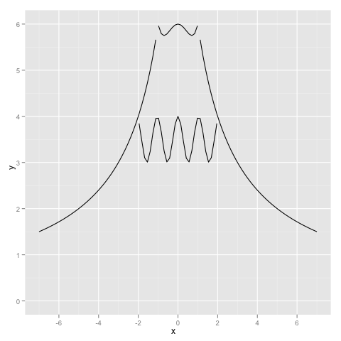
ggplot2だと線がうまくつながらなかった。

Ggplot2: Elegant Graphics for Data Analysis (Use R!)
Hadley Wickham
Springer-Verlag New York Inc (C) / ￥ 5,259 ( 2009-08-30 )

dose-responseカーブのあてはめをしたり、解析をしたりするためのdrcというパッケージを触ってみたのでメモ。

ryegrass(イネ科の牧草)におけるフェルラ酸の効果を調べたというデータを4パラメータのlog-logistic functionであてはめる。

ryegrass.m1<-drm(ryegrass, fct = LL.4())
plot(ryegrass.m1)

Rでのネットワーク分析用ライブラリの使い方が知りたい場合には良い本。snaとigraphの使い方がまとまっている。

第3章の「ネットワーク構造の諸指標」(密度、推移性、相互性)と第4章の「中心性」は役に立った。

ネットワーク分析 (Rで学ぶデータサイエンス 8)
鈴木 努
共立出版 / ￥ 3,465 ()
在庫あり。

いちおう、どういう場合にその手法が必要になるのかといったことをさらっと載せてからigraph,snaのサンプルコードを載せているが、本書はRの使い方がメインなので、特定の分野用のネットワーク分析の本もあわせて読んだほうがいいと思う。

igraphはRとPythonのbindingがあるのにチュートリアルがほとんどなさげなので、ネットワーク分析の本があると手っ取り早く知れて良い。

ネットワーク分析 (Rで学ぶデータサイエンス 8)
鈴木 努
共立出版 / ￥ 3,465 ()
在庫あり。

クリーク探索

こんなネットワークからクリークを探してみる

g <-matrix(c(0,1,1,0,1,0,0,1,0,1,0,0,0,1,1,1,0,1,1,1,0,0,
             0,1,0,1,1,1,1,0,1,1,0,1,0,0,0,1,1,1,0,0,0,1,
             0,1,0,0,0),nrow=7,ncol=7,byrow=TRUE) 
a <- graph.adjacency(g)
maximal.cliques(a)
[[1]]
[1] 0 1 2

[[2]]
[1] 1 6

[[3]]
[1] 0 2 4

[[4]]
[1] 2 3 4 5

[[5]]
[1] 3 6

追記 100818

Pythonの場合

a = [[0,1,1,0,1,0,0],
[1,0,1,0,0,0,1],
[1,1,0,1,1,1,0],
[0,0,1,0,1,1,1],
[1,0,1,1,0,1,0],
[0,0,1,1,1,0,0],
[0,1,0,1,0,0,0]]

g = GraphBase.Adjacency(a,mode=ADJ_UNDIRECTED)
g.maximal_cliques() # [(0, 1, 2), (1, 6), (0, 2, 4), (2, 3, 4, 5), (3, 6)]
g.largest_cliques() # [(2, 3, 4, 5)]

昨日の化合物の類似性ネットワークのやつは何がメリットなのかなぁと考えてみたけど、一つにはedgeの数を自由に決められるあたりなんじゃないかと。あんまり低い閾値だとなんでもかんでもつながって何見てるかわからんし、逆に厳しい閾値にしちゃうとシングルトンばかりになっちゃうし。

というわけで、プロット欠かせてそれ見て閾値決める必要はあるんだろうなと。最終的にはeddgesの数とか、ノードあたりに生えているedgeの数の平均とかを統計的に処理して自動で閾値を決めるのが楽なんだろうけど、、、（一般的な方法あるのかな？）。X-meansに倣って、BICとかAIC使ってみようかなぁ。

で、プロット描いた。最初に書いたコードがナイーブすぎて遅くていらっときたので書き直した。まだかなり遅いけど、耐えられるのでこれでよしとした。

import pybel

mols = list(pybel.readfile("sdf", "pc_sample.sdf"))
fps = [x.calcfp() for x in mols] 

similarity_matrix = []
for i in range(len(fps)):
    for j in range(i+1,len(fps)):
        similarity = fps[i] | fps[j]
        similarity_matrix.append(similarity)

threshold = 0.0
print "threshold\tnodes"
while threshold < 100:
    t = threshold / 100.0
    new_matrix = [e for e in similarity_matrix if e > t]
    nodes = len(new_matrix)
    print "%2.1f\t%d" % (threshold, nodes)

    similarity_matrix = new_matrix
    threshold += 0.1

あとはRで

library(ggplot2)
nodes <- read.table("xxxx",header=T)
qplot(threshold,edgess, data=nodes, log="y")
dev.copy(device=png,filename="xxxxxx")
dev.off()

node数が1158なのでedgeの数が10000から100あたりの間でちょうどいい閾値を探したいんだけど、これだけじゃわからん。やっぱシングルトンの数とかノードあたりに生えているエッジ数の平均とか数えないとだめかな。

the Journal of Statistical SoftwareにPypeRというpythonからRを使うパッケージの論文が出てた。

Most Bioconductor tools are presented as R packages. Therefore, R can be a good complement to Python in bioinformatics computation.

メモリの使用量が低く抑えられる感じ？RPyやRPy2とかと比較している

でも、なんかpythonの中でRの構文埋め込んでるみたいな感じだなぁ。PypeRってのはそういうことなのかな。

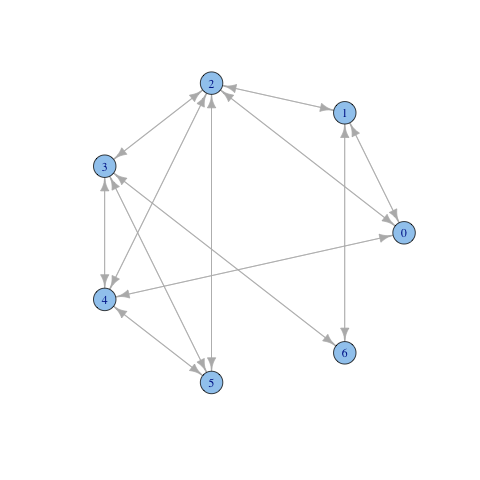
Bioinformatics Programming Using Python
Mitchell L. Model
Oreilly & Associates Inc / ￥ 5,584 ()
在庫あり。

Statistical Bioinformatics: with R
Sunil K. Mathur
Academic Press / ￥ 5,605 ()
在庫あり。

Building Bioinformatics Solutions: With Perl, R and Mysql
Conrad Bessant,Ian Shadforth,Darren Oakly
Oxford Univ Pr (Txt) / ￥ 4,163 ()
在庫あり。

R Programming for Bioinformatics (Chapman & Hall/Crc Computer Science & Data Analysis)
Robert Gentleman
Crc Pr I Llc / ￥ 6,532 ()
通常2～5週間以内に発送

Rにおける高階関数はCommon Higher-Order Functions in Functional Programming Languagesにあるように一通りそろっている

Reduce uses a binary function to successively combine the elements of a given vector and a possibly given initial value. Filter extracts the elements of a vector for which a predicate (logical) function gives true. Find and Position give the first or last such element and its position in the vector, respectively. Map applies a function to the corresponding elements of given vectors. Negate creates the negation of a given function.

foldl,foldrも簡単

foldl <- function(f,x,i){Reduce(f,x,i)}
foldr <- function(f,x,i){Reduce(f,x,i,right=TRUE)}

実行してみる

> foldl("-",list(1,2,3),1) # ((1-1)-2)-3
[1] -5
> foldr("-",list(1,2,3),1) # 1-(2-(3-1))
[1] 1

あとRの高階関数は大文字で始める規則にでもなってんのかな？

Rの基礎とプログラミング技法
U.リゲス
シュプリンガー・ジャパン(株) / ￥ 3,675 ()
通常1～4週間以内に発送

Rでパッケージ作るときにパッケージ変数として扱いたいものを

pit_dir <- file.path(Sys.getenv("HOME"),".pit")
pit_config <- file.path(pit_dir,"pit.yaml")
pit_profile_file <- NULL

と先頭に書いておきたいのだけどNAMESPACEファイルを作成すると

> library(pit)
 要求されたパッケージ yaml をロード中です 
> pit.switch("test")
 以下にエラー pit.switch("test") : 
   'pit_profile_file' に対するロックされたバインディングの値は変更できません 

とでる。ちなみにpit.switchはこれ

pit.switch <- function(name=NULL){
  if(is.null(name)) name <- "default"
  pit_profile_file <<- file.path(pit_dir, paste(name, ".yaml", sep=""))
  config <- pit.config()
  ret <- config$profile
  config$profile <- name
  write(as.yaml(config),pit_config)
  if(name != ret) write(paste("Profile switch to",name,"from",ret), stderr())
  return(ret)
}

環境をとってきてunlockBindingすればいいんだろうなぁと思うんだけどやり方が分からなくて、

pit_dir <- file.path(Sys.getenv("HOME"),".pit")
pit_config <- file.path(pit_dir,"pit.yaml")
#pit_profile_file <- NULL
assign("pit_profile_file",NULL,pos =".GlobalEnv")

とやって、直接大域環境に変数をセットしてるんだけど、これって本当はどうするのがいいんだろうか？

Rの基礎とプログラミング技法
U.リゲス
シュプリンガー・ジャパン(株) / ￥ 3,675 ()
通常1～4週間以内に発送

追記10.07.08

環境オブジェクトを作るという方法もあるそうなので、こっちでやってみた。

pit_dir <- file.path(Sys.getenv("HOME"),".pit")
pit_config <- file.path(pit_dir,"pit.yaml")
conf<-new.env()
conf$pit_profile_file <- NULL

こっちのほうが精神衛生上よろしいかも。それにしてもRの環境ってなんだろか？Lispみたいな感じで考えとけばいいのかな？あとでソースコードを探ってみよう。

参考

• 一次的作業環境の使用 new.env(TRUE,NULL)
• MooseでLispを実装してみる(ラムダリストと変数の局所化)

Shiga.Rお疲れ様でした。内容盛りだくさんで面白かったのと、色々な人に出会えて有意義でした。というかこの三日間は充実してた。

plotter.Rはpit使わなくても、usernameとpassword直接入力すれば動きます。twitpicのAPIを使っているので、画像をポストしつつtwitterに投稿するようになっている(デモの時にはtwitterにはポストされなかったけど)。

帰りの新幹線でRいじってたので、irisをMDSとspeで次元縮約したのをポストしてた。

require("RCurl")
require("pit")
profile=pit.get("twitter.com",require=list(username="username",password="password"))

pweet <- function(status){
  tempfile <- tempfile(pattern = "file", tmpdir = tempdir())
  dev.copy(device=png,filename=tempfile)
  dev.off()
  twitpicreq <- "http://twitpic.com/api/uploadAndPost"
  params = list(media=fileUpload(filename=tempfile),username=profile$username,password=profile$password,message=status)
  twitpicresponse <- postForm(twitpicreq,.params = params)
}

あと、R版pit

R CMD INSTALL pit_0.8.tar.gz

でインストールできます。ただ、pit.setするときにエディタが起動するように鳴っているのだけど、terminalでRを起動しているときにはいいのだけど、それ以外の時（RのコマンドインターフェースとかESS）ではエディタが立ち上がらずおかしなことになるので、そこのとこをちょっとどうにかしないといけない。

あと、NAMESPACEというファイルを作ったら<<-で変数の代入が出来なくて、面倒になってファイルを削除してしまったのだけど、今日話を聞いてたらなんとなくやり方がわかったのであとでなおす。

違うことをしていたらPSM:PSM: Non-Linear Mixed-Effects modelling using Stochastic Differential Equationsという面白そうなパッケージを見つけたのでサンプルで遊んでみた。

集団から個人をサンプリングしてきてシミュレーションできるという理解でいいのかな？

確率微分方程式―入門から応用まで
ベァーント エクセンダール
シュプリンガー・フェアラーク東京 / ￥ 4,935 ()
在庫あり。