
微分方程式を解くためにodesolveを利用する。初期値の与えかたとか、ぐるぐる回していくイメージをつかむのに微妙に時間がかかったが、覚えてしまうと簡単な方程式を解かせたりシミュレーションするのには楽になる。
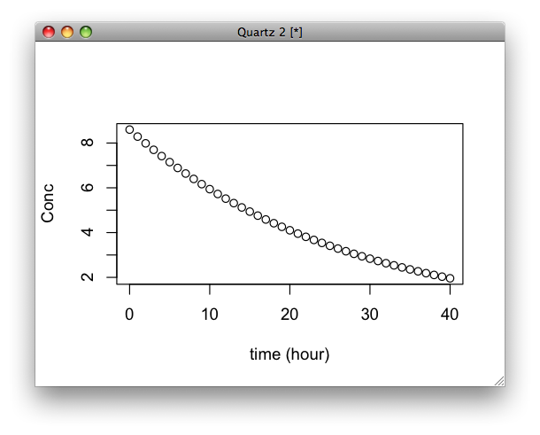
設問1
吸収過程を考えないコンパートメントモデル
library(odesolve)
params <- c(kel = 0.037)
times <- c(0,(1:40))
dydt <- function(t,y,p){
  kel <- p['kel']
  y <- -kel*y
  list(c(y))
}
y <- lsoda(c(y = 8.6),times,dydt,params)
plot(y,ylab="Conc",xlab="time (hour)")
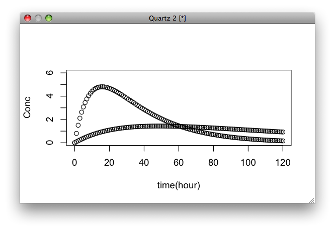
設問2&3
今度は吸収過程を考える。設問3は吸収速度定数を1/10にした時にどういう挙動を示すか。
params <- c(kel = 0.037,ka = 0.1, D = 5000, V = 580)
times <- c(0,(1:120))
dydt <- function(t,y,p){
  kel <- p['kel']
  ka <- p['ka']
  D <- p['D']
  V <- p['V']
  y <- ka * (D/V) * exp(-ka*t) -kel*y
  list(c(y))
}
y <- lsoda(c(y = 0),times,dydt,params)

params2 <- c(kel = 0.037,ka = 0.01, D = 5000, V = 580)
y2 <- lsoda(c(y = 0),times,dydt,params2)

plot(y,ylim=c(0,6),ylab="Conc",xlab="time(hour)")
par(new=T)
plot(y2,ylim=c(0,6),axes=F,xlab="",ylab="")
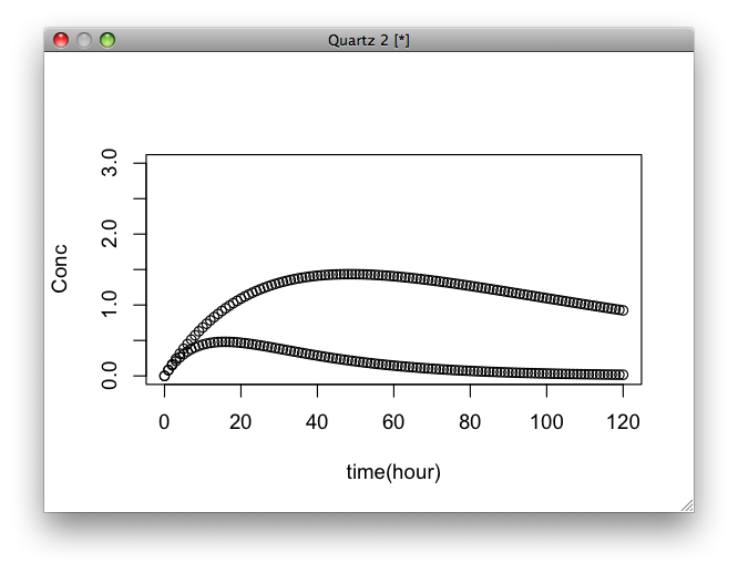
今回バイオアバイラビリティ(F)を1とおいているが、これを変化させた時の挙動も気になるのでやってみた。設問の式にFを組み込んでF=0.1とした時の結果
dydt2 <- function(t,y,p){
  kel <- p['kel']
  ka <- p['ka']
  D <- p['D']
  V <- p['V']
  F <- p['F']
  y <- ka * (D/V) * F * exp(-ka*t) -kel*y
  list(c(y))
}

params3 <- c(kel = 0.037,ka = 0.1, D = 5000, V = 580, F = 0.1)
y3 <- lsoda(c(y = 0),times,dydt2,params3)

plot(y2,ylim=c(0,3),axes=F,xlab="time(hour)",ylab="Conc")
par(new=T)
plot(y3,ylim=c(0,3),axes=F,xlab="",ylab="")
あーなるほど、そうだよなぁと一人で妙に納得したのであった。
 ファーマコキネティクス―演習による理解