
演習の本をRでこなしていくことにした。
 ファーマコキネティクス―演習による理解
設問1
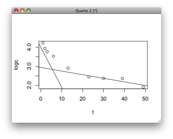
β層の消失速度をもとめて、それを用いてα層の消失速度を決定する。
t <- c(1,2,3,6,13,23,30,39,49)
c <- c(68.2, 51.1, 43.2, 34.0, 18.3, 11.5, 10.7, 10.6, 6.78)
23時間からの濃度からβ層の消失速度を求める
logc <- log(c)
result <- lm(logc[6:9] ~ t[6:9])
coef(result)
 (Intercept)      t[6:9]
 2.93770720 -0.01888941
β層の消失速度が決まったので、次は23時間までの濃度からβ層の寄与を引いた濃度からα層の消失速度を決定する
beta <- function(t){exp(2.937707-0.01889*t)}
alogc <- c[1:5] - beta(t)[1:5]
aresult <- lm(alogc ~ t[1:5])
これでα層β層それぞれの消失速度がもとまる
result

Call:
lm(formula = logc[6:9] ~ t[6:9])

Coefficients:
(Intercept)       t[6:9]
    2.93771     -0.01889

aresult

Call:
lm(formula = alogc ~ t[1:5])

Coefficients:
(Intercept)       t[1:5]
     3.9916      -0.2088
求めるモデルは
exp(3.9916-0.2088*t)+exp(2.937707-0.01889*t)
設問2
ラフに求めたA,B,alpha,betaを初期値として最小自乗法でフィッティングを行う。1exp,2expでやってみて、どっちのあてはまりがよいか考える
t <- c(1,2,3,6,13,23,30,39,49)
conc <- c(68.2, 51.1, 43.2, 34.0, 18.3, 11.5, 10.7, 10.6, 6.78)
dat <- data.frame(conc,t)
result <- nls(conc ~ a*exp(-alpha*t),start=list(a=50,alpha=0.045))
summary(result)

Formula: conc ~ a * exp(-alpha * t)

Parameters:
      Estimate Std. Error t value Pr(>|t|)
a     63.26990    5.39879  11.719 7.45e-06 ***
alpha  0.08359    0.01777   4.706  0.00219 **
---
Signif. codes:  0 ‘***’ 0.001 ‘**’ 0.01 ‘*’ 0.05 ‘.’ 0.1 ‘ ’ 1

Residual standard error: 6.608 on 7 degrees of freedom

Number of iterations to convergence: 14
Achieved convergence tolerance: 7.74e-06

f <- function(t){63.2699*exp(-0.0836*t)}
plot(f,0,50,xlim=c(0,50),ylim=c(0,70),xlab="Time",ylab="Conc")
par(new=T)
plot(t,conc,xlim=c(0,50),ylim=c(0,70),axes=F,xlab="",ylab="")
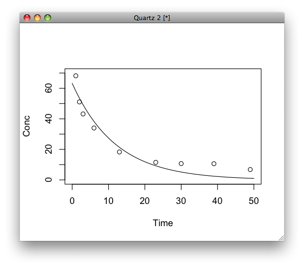
一層の消失モデルだと特に遅い時間の当てはめが悪い。ちなみにRだとAIC関数使えば適合度がでる。
t <- c(1,2,3,6,13,23,30,39,49)
conc <- c(68.2, 51.1, 43.2, 34.0, 18.3, 11.5, 10.7, 10.6, 6.78)
dat <- data.frame(conc,t)
result <- nls(conc ~ a*exp(-alpha*t)+b*exp(-beta*t),start=list(a=50,alpha=0.277,b=20,beta=0.0198))
summary(result)
f <- function (t){55.75*exp(-0.3769*t)+29.157*exp(-0.03189*t)}
plot(f,0,50,xlim=c(0,50),ylim=c(0,70),xlab="Time",ylab="Conc")
par(new=T)
plot(t,conc,xlim=c(0,50),ylim=c(0,70),axes=F,xlab="",ylab="")
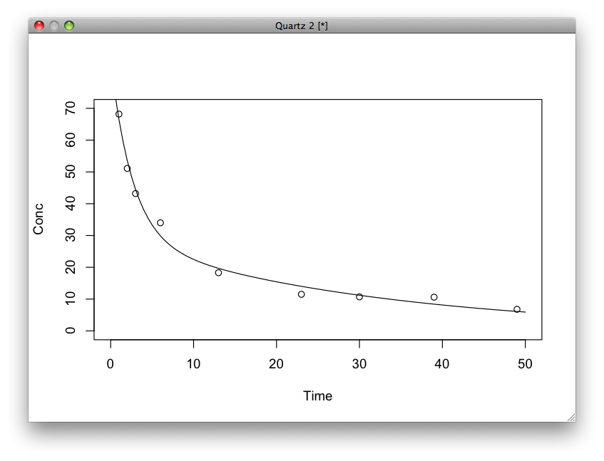
プロットするときにpar関数で上書きするのと、xlim,ylimを明示して軸をきちんとそろえつつ、目盛やタイトルを上書きして重ねないように気をつける。